6  t-tests

6.1 Intro

In the early 1900s, William Sealy Gosset joined Guinness, then the world’s largest brewery. Guinness hired scientifically trained brewers and gave them latitude to pursue research that improved the product. As production scaled, quality control mattered: a pint should taste the same in Dublin as in Detroit. Until then, hop quality was judged mostly by appearance and smell, which was unreliable. Chemical assays could measure ingredients, but the core problem was statistical. Inference relied on the normal (Z) distribution, which works well when samples are large enough for a normal approximation. In practice, Guinness could not destroy large volumes of beer or ingredients just to test them.

Gosset set out to quantify the extra uncertainty introduced by small samples. How much wider is the error around an estimate when \(n=10\) instead of \(n=1000\)? He derived a new sampling distribution that accounts for small-sample variability, now known as the Student’s \(t\) distribution. Because Guinness restricted external publications, he published the 1908 paper under the pseudonym “Student” (Student 1908). That is why we still say Student’s \(t\)-test. The core idea you will use today is the same: measure a signal, scale it by its standard error, and compare the resulting \(t\) to the appropriate \(t\) distribution for your \(n-1\) degrees of freedom.

Why this matters. We often compare a sample mean to a reference (drinking-water standard, historical average) or compare two conditions (before/after, site A vs site B). A t-test asks whether the observed difference is larger than you would expect from sampling variation alone, given your \(n\) and variability.

Three common t-tests you will use.

1. One-sample t-test. Compare a sample mean to a target (\(\mu_0\)).
2. Paired t-test. Compare before/after (or matched) measurements on the same units by running a one-sample t on the differences.
3. Independent-samples t-test (also called two-sample t-test) Compare means from two groups measured on different units. The pooled version assumes the two groups have similar spread; Welch’s version (Welch 1947) does not, and it is what R’s t.test() runs unless you set var.equal = TRUE.

TipTip: What you will report

Always report:

• the effect size (mean difference)
• a 95% CI
• the test statistic with its df
• the \(p\)-value

Example: “Mean change was -0.42 units (95% CI [-0.73, -0.11]; t(11) = -2.92; p = 0.014).”

6.2 Signal over noise, for a mean

Chapter 4 introduced the general shape of a test statistic: the effect you observed, divided by an estimate of how much it could move by chance.

\[\text{statistic}=\frac{\text{effect}}{\text{error}}\]

The \(t\)-test is the first place we fill that in with real quantities. The effect is the distance between the sample mean and the value \(H_0\) names. The error is not the raw standard deviation, though: it is the standard error, \(s/\sqrt{n}\), because what varies from study to study is the mean, not an individual observation.

\[t = \frac{\text{effect}}{\text{standard error}} = \frac{\bar{x} - \mu_0}{s / \sqrt{n}}\]

We now turn that ratio into a test statistic for a single mean.

6.3 One-sample t-test

Use a one-sample \(t\) when you want to test whether a sample mean differs from a reference value (\(\mu_0\)). The question: is the observed difference bigger than you’d expect from sampling variability, given \(n\) and your sample SD \(s\)?

\[t = \frac{\bar{x}-\mu_0}{s/\sqrt{n}}, \qquad df = n-1\]

After calculating \(t\) from our data, we compare the observed \(t\) to a \(t\) distribution with \(n-1\) degrees of freedom to get a \(p\)-value and a decision at \(\alpha\).

6.3.1 Comparing \(z\) and \(t\)

When the population SD is known (or the sample is large enough that \(s\) is close to \(\sigma\)), the ratio is called \(z\). When the SD is estimated from the data, the ratio is called \(t\).

Under a known population SD (\(\sigma\)), the standardized mean uses the \(z\) statistic: \[z = \frac{\bar{x}-\mu_0}{\sigma/\sqrt{n}}\]

When \(\sigma\) is unknown (the usual case), we estimate it with the sample SD (\(s\)) and use the \(t\) statistic: \[t = \frac{\bar{x}-\mu_0}{s/\sqrt{n}}, \qquad df = n-1\]

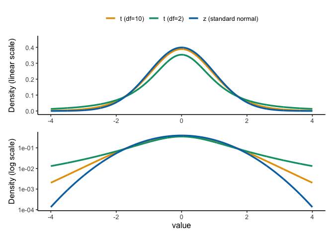
Because \(s\) varies from sample to sample, the \(t\) distribution has heavier tails than the standard normal. As \(n\) grows, \(s\) stabilizes and \(t\) converges to \(z\).

Figure 6.1: Normal (\(z\)) vs \(t\) distributions: on a linear scale (top), tail differences look small; on a log scale (bottom), the heavy tails of small-\(n\) \(t\) are clear.

TipTip: When is \(z\) appropriate?

If the population SD \(\sigma\) is known and the sampling distribution of the sample mean is (approximately) normal, use \(z\). In practice, \(\sigma\) is rarely known, so we use \(t\) with \(s\) and \(df=n-1\).

Rule of thumb. For two-tailed tests at \(\alpha=0.05\):

• \(z\) uses critical values \(\pm 1.96\).
• \(t\) is a bit wider for small \(n\) (e.g., \(df=9 \Rightarrow \pm 2.262\); \(df=29 \Rightarrow \pm 2.045\)), and approaches \(\pm 1.96\) as \(n\) increases.

6.3.2 Degrees of freedom

Every \(t\) formula so far has carried \(df = n-1\) alongside it, and Figure 6.1 drew a different \(t\) curve for each \(df\). That number is the degrees of freedom. It is also the number in parentheses whenever a \(t\)-test is reported, as in \(t(9) = 1.94\).

For one-sample and paired \(t\)-tests, \(df = n-1\). A sample of 10 has \(df=9\).

Degrees of freedom counts how many values are still free to vary once something has been estimated from the data. Consider three numbers with a mean of 2: pick the first two freely, say 51 and \(-3\), and the third number is no longer free. It has to be \(-42\) for the mean to come out to 2. Two of the three numbers had freedom; the third didn’t. That’s \(df=n-1=2\) for three numbers.

In a \(t\)-test, the mean is the thing estimated, and the \(df\) tells you how much information is left for estimating the spread, \(s\). With few degrees of freedom, \(s\) can land well above or below \(\sigma\), so large \(t\) values turn up more often and the \(t\) curve has heavier tails. As \(df\) grows, \(s\) settles close to \(\sigma\) and the \(t\) curve approaches the normal. That is why each \(df\) gets its own curve.

Simulating how degrees of freedom affects the \(t\) distribution.

We can see the effect of degrees of freedom directly by simulating the \(t\) distribution at two different sample sizes. Figure 6.2 compares \(df=9\) (a sample of 10) to \(df=100\) (a much larger sample).

Figure 6.2: The width of the t distribution shrinks as sample size and degrees of freedom (from 9 to 100) increases.

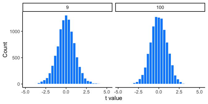
As degrees of freedom increase, the \(t\) distribution gets taller in the middle and narrower in the tails. With more data the sample SD is a more reliable stand-in for \(\sigma\), so \(t\) behaves more like \(z\).

6.3.3 What t represents

Whether we use \(z\) or \(t\), the ratio asks the same question: how far is the mean from the reference in SE units?

\(t\) expresses how far a sample mean is from the hypothesized mean, in standard error units (signal over noise):

\[t = \frac{\bar{x}-\mu_0}{s/\sqrt{n}}\]

\(t\) can be positive or negative depending on direction. Under \(H_0\), \(t \sim t_{(df=n-1)}\).
Rule of thumb: at \(df\approx 20\), \(|t|\) beyond about 2 occurs less than 5% of the time under \(H_0\) (two-tailed, \(\alpha=.05\)). With smaller \(df\) the cutoff is higher, as the critical values above show.

NoteNote: Standard error, again

Remember that \(s/\sqrt{n}\) is the standard error (SE), the standard deviation of the sampling distribution of the sample mean.

Let’s see how \(t\) values behave when samples really come from the null hypothesis. Under the null hypothesis, \(t\) follows a \(t\) distribution with \(df = n-1\).

Figure 6.3: Histogram of 1,000 simulated \(t\) values (\(n=10\)) drawn from a population with \(\mu_0=0\). Most \(t\)s cluster near 0; large positive or negative values are rare.

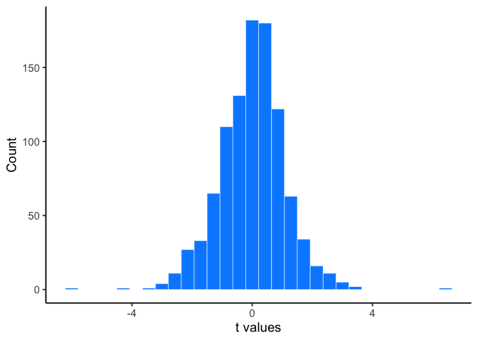
Takeaway: \(t\) measures how far the sample mean is from the null expectation, scaled by its uncertainty. Under \(H_0\) it follows a known \(t\) distribution, so we can check how often chance alone would produce a \(t\) as large as ours.

6.3.4 Calculating t from data

Let’s calculate a one-sample \(t\) statistic step by step using a short example. Ten students each took a 5-question true/false quiz (50% expected by chance). Their scores (percent correct) are:

Scores: 50, 70, 60, 40, 80, 30, 90, 60, 70, 60

By hand, the standard error of the mean is the sample SD divided by the square root of \(n\):

\[\text{SE} = \frac{s}{\sqrt{n}} = \frac{17.92}{\sqrt{10}} = 5.67\]

And \(t\) is the difference between the sample mean (61) and the reference value (50, chance level), divided by that SE:

\[t = \frac{\bar{x}-\mu_0}{SE} = \frac{61-50}{5.67} = 1.94\]

We can confirm this with a single R command, t.test(scores, mu = 50):

Results: \(t(9)=1.94\), \(p=0.0842\); mean \(=61\) (95% CI [48.18, 73.82]).

Interpretation: The mean (61%) is above chance (50%), but the difference is not statistically significant at \(\alpha=.05\).

Assumptions check: Observations are independent, and the 10 scores are approximately normal, which is sufficient for a one-sample \(t\)-test.

6.3.5 Assumptions, and what to do when they don’t hold

Every test in this book has assumptions. Assumptions are conditions that need to be roughly true for the math behind the test to be trustworthy. There are two different kinds of assumptions.

The universal assumption. Every test in this book, including the nonparametric tests in Chapter 7, assumes your observations are independent (in paired designs, the pairs) and came from a sound study design (a fair sample, not one that systematically favors certain values). This assumption is so constant that from here on, we won’t re-list it test by test. Keep it in the back of your mind, but if an exam or homework question asks you to “list the assumptions of this test,” this isn’t the answer they’re looking for.

Test-specific assumptions. These come from how a particular test’s math actually works, and they differ test to test. For the one-sample and paired \(t\)-tests, the specific assumption is approximate normality of the outcome itself (one-sample) or of the difference scores (paired). The \(t\)-distribution we’ve been using to get \(p\)-values is derived assuming the sampling distribution of the sample mean is normal. If your data are badly skewed and your sample is small, that assumption fails, and the \(p\)-value may not be the true probability of a result this extreme under \(H_0\).

How worried should you be? It depends enormously on \(n\). With a large sample, the Central Limit Theorem does a lot of the work for you. The sampling distribution of the sample mean tends toward normal even when individual observations are skewed, so the \(t\)-test is fairly robust to non-normality once \(n\) is reasonably large. A lot of environmental data, particularly field data, instead comes from small samples that are also skewed. Examples include a handful of expensive water samples, a short list of monitoring wells, or the five plots you had time to visit before the storm rolled in. A \(t\)-test’s answer becomes questionable when the sample is small and the data are also non-normal.

What to do about it. First, look at your data. A histogram or a QQ-plot will usually tell you whether “approximately normal” is a reasonable description or a stretch. You can also run a formal normality test, the Shapiro-Wilk test (shapiro.test() in R), which tests \(H_0\): the data came from a normal distribution. Treat it as one more piece of evidence rather than a strict gate though: with a small sample, exactly when a violation matters most, it has low power and will often say “no problem” even when there is one. If your data look far from normal and your sample is small, you have another option: a nonparametric test, which does not assume normality. You’ll meet these nonparametric alternatives in the next chapter, once we’ve covered all three t-test forms below.

6.3.6 How does t behave?

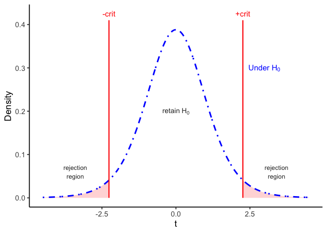
Extreme sample means are unlikely if \(H_0\) is true, which is why large \(|t|\) values are rare. Returning to that rule of thumb, values of \(t\) beyond roughly \(-2\) or \(+2\) occur less than 5% of the time under the null when \(df \approx 20\). That’s the foundation of the decision rule for \(t\) tests: if your observed \(t\) lies in those rare tails, you reject \(H_0\).

With the single \(t\) from our sample, we can check Figure 6.4 to see whether a \(t\) that size is likely or unlikely by chance alone.

Figure 6.4: Two-tailed rejection regions at \(\alpha=.05\) for \(t_{(df=9)}\). The shaded tails beyond the red critical values mark unlikely values under \(H_0\).

6.3.7 Interpreting \(t\)

We’re asking whether our \(t\)-value could plausibly have come from the null distribution: the distribution of \(t\)-values we’d see across many samples of size 10, if the true mean were exactly 50 (chance level). Figure 6.5 shows what that distribution looks like, at \(df=9\).

Figure 6.5: A distribution of \(t\)-values that can occur by chance alone, when there is no difference between the sample and a population

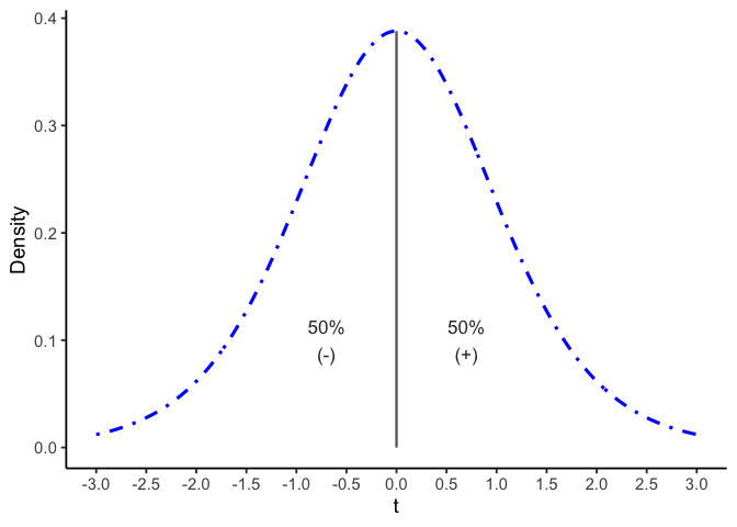
\(t\) is most likely to land near zero, which makes sense: this is the distribution of no differences, so most of the time chance alone won’t push it far from 0. Because the distribution is symmetric, a \(t\)-value from the null distribution is just as likely to be positive as negative.

That symmetry gives us a few basic probabilities for free:

1. \(t\) is always zero, positive, or negative, so \(p(t=0 \text{ or } t>0 \text{ or } t<0) = 1\).
2. \(p(t \geq 0) = .5\): half of all \(t\)-values are zero or greater.
3. \(p(t \leq 0) = .5\): half are zero or smaller.

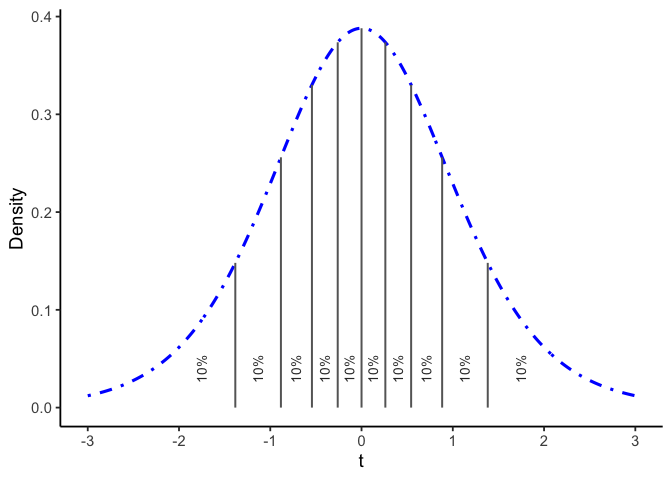
We can get more precise than a 50/50 split. Figure 6.6 divides the same distribution into ten regions, each containing 10% of the distribution. Notice the regions get wider out in the tails: since most \(t\)-values cluster near 0, it takes a wider interval out there to capture the same 10%.

Figure 6.6: Splitting the t distribution up into regions each containing 10% of the \(t\)-values. The width between the bars narrows as they approach the center of the distribution, where there are more \(t\)-values.

For example:

1. \(t \leq -1.38\): \(p = 10\%\)
2. \(-1.38 \leq t \leq -0.88\): \(p = 10\%\)
3. \(-0.88 \leq t \leq -0.54\): \(p = 10\%\)
4. \(t \geq 1.38\): \(p = 10\%\)

Each range captures the same 10% of the distribution, even though the ranges themselves are different widths.

6.3.8 Getting the p-values for \(t\)-values

Older textbooks listed these values in a table at the back of the book. R, Excel, and online calculators all work; you’ll get hands-on practice with this in lab, both with software and by simulation.

Software needs two things from you to compute a \(p\)-value: the degrees of freedom, which you already have, and whether the test is one-tailed or two-tailed, which comes next.

6.3.9 One-tailed vs. two-tailed, applied

Chapter 4 introduced the concept: a two-tailed test asks whether \(\mu\) differs from \(\mu_0\) in either direction, while a one-tailed test commits to one direction in advance, and is only justified when a result in the other direction would lead to the same action as no result at all. For a \(t\)-test, that choice changes the critical value, and therefore the \(p\)-value, for the exact same data.

For our quiz-score example (\(df=9\)), a one-tailed test only needs to clear 5% of the distribution on one side. A two-tailed test has to clear 2.5% on each side, which pushes the critical value farther out:

Figure 6.7: One-tailed critical value at df=9: t-values of 1.83 or greater occur 5% of the time.

Figure 6.8: Two-tailed critical values at df=9: t-values beyond ±2.26 occur 5% of the time total, 2.5% in each tail.

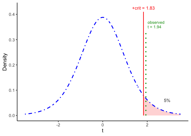
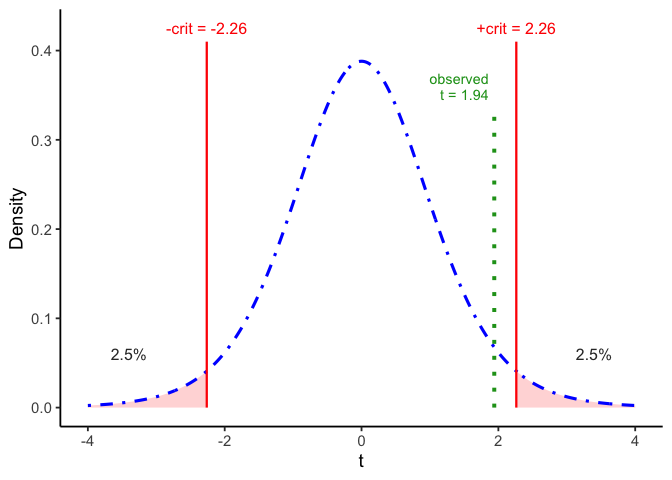
Applied to our actual result, \(t(9) = 1.94\): the one-tailed \(p\) is .042, the two-tailed \(p\) is .084, exactly double, since a two-tailed test counts the matching extreme region on both sides instead of just one. Here the choice actually changes the decision: one-tailed, this result is significant at \(\alpha=.05\); two-tailed, it isn’t. That’s exactly why a one-tailed test has to be justified by your theory before you see the data, not chosen afterward because it gives the answer you wanted.

6.3.10 Which one should you use?

The rule is Chapter 4’s, unchanged: default to two-tailed, and go one-tailed only when a result in the opposite direction would lead you to do the same thing as no result. With a \(t\)-test you can see the difference in the critical value: at the same \(\alpha\), the one-tailed \(t_{crit}\) is closer to 0 than the two-tailed one.

6.4 Paired t: before/after or matched

When the same units are measured twice (before/after, matched pairs), the question is whether they changed. The natural data unit is the within-unit difference.

Design in this worked example. Ecologists measured soil moisture at 20 field plots before wetland restoration and again one year later, to see whether restoration increased moisture enough to support plant reestablishment and carbon sequestration. Figure 6.9 shows the design.

Figure 6.9: A paired design. The dashed boxes and the note underneath mark the feature that defines it: there is one set of 20 plots, measured on two occasions, not two separate samples.

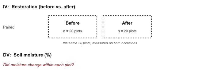
The dashed boxes mark what makes this design paired. In every design so far the boxes held different units, and the test compared one set against another. Here both boxes hold the same 20 plots, which is what makes the design paired and what lets us subtract.

Define differences and their meaning. Choose an order and stick to it:

• \(d_i = \text{After}_i - \text{Before}_i\)
• \(d_i>0\): plot had more soil moisture after restoration (increase)
• \(d_i<0\): plot had less soil moisture after restoration (decrease)

This subtraction cancels between-plot variability (some plots are naturally wetter than others) and focuses on within-plot change.

Test on differences (paired \(t\)). Compute one difference per plot, then run a one-sample \(t\) against 0:

\[\bar d=\frac{1}{n}\sum_{i=1}^n d_i, \quad s_d=\text{SD}(d_1,\ldots,d_n), \quad t = \frac{\bar d - 0}{s_d/\sqrt{n}}, \quad df=n-1.\]

The sign of \(t\) matches \(\bar d\) and your difference direction.

Full sample effect. With all 20 plots, \(\bar d\) is similar to its value in a 5-plot subset, but \(s_d/\sqrt{n}\) gets smaller as \(n\) grows, so \(t\) increases.

What to report. \(\bar d\) (the mean change), a 95% CI, \(t(df)\), and \(p\). Optionally add a standardized effect (Cohen’s \(d=\bar d/s_d\)).

R pointers (you’ll do this in lab).

• Compute differences: d <- after - before
• Paired \(t\): t.test(d, mu = 0) or t.test(after, before, paired = TRUE)
• CI for \(\bar d\): from the t.test output

6.4.1 Calculate t

To calculate \(t\) for a paired-samples \(t\)-test, we use the one-sample \(t\)-test formula from the previous section, applied to the difference scores instead of raw scores. The paired-samples \(t\)-test is a one-sample \(t\)-test on a single group of numbers, the differences.

Let’s find \(t\) for the mean difference scores:

plot	Before	After	differences	diff_from_mean	Squared_differences
1	18	21	3	0.2	0.0400000000000001
2	22	26	4	1.2	1.44
3	16	22	6	3.2	10.24
4	25	29	4	1.2	1.44
5	21	18	-3	-5.8	33.64
Sums	102	116	14	0	46.8
Means	20.4	23.2	2.8	0	9.36
				sd	3.421
				SE	1.53
				t	1.83006535947712

If we did this test using R, we would obtain almost the same numbers (there is a little bit of rounding in the table).

Paired t-test on 5 restoration plots

Mean difference	t	df	p-value
2.8	1.83	4	0.141

Our t-test results are: t(4) = 1.83, p = .141.

The sign of \(t\) matches the sign of the mean difference (ours was \(+2.8\) percentage points), so soil moisture increased on average, as \(\bar d\) showed. Getting a \(p\)-value from this \(t\), and choosing one-tailed vs. two-tailed, works exactly like it did for the one-sample case (see the One-sample \(t\)-test section above). Two-tailed, \(p=.141\), which is not significant. This five-plot sample is too small to rule out chance.

6.4.2 Scaling to the full sample

The five plots above are a subset of the full restoration study, which measured all 20 paired plots. With only \(n=5\), \(t(4)=1.83\) wasn’t enough to distinguish the observed increase from chance (\(p=.141\)).

Paired t-test on all 20 restoration plots

Mean difference	t	df	p-value
1.9	2.5	19	0.022

At \(n=20\), \(t(19) = 2.5\), \(p =0.022\): significant. The mean difference (1.9 percentage points) is in the same range as the 5-plot subset suggested. The standard error shrank enough with the larger sample to rule out chance, so the extra plots gave more power to detect a real effect.

6.5 Two independent groups

The independent-samples \(t\)-test is the third and last design in this chapter. The logic is the same as the one-sample and paired cases: a mean difference divided by an estimate of its variability. Only the research design is different.

Use an independent-samples \(t\)-test for a between-subjects design: different people or units in each condition, each measured once. With two groups of 10, that’s 20 people total, none of them paired. Without repeated measures on the same unit, there’s no meaningful way to subtract scores between conditions the way the paired \(t\)-test does.

The numerator works the same way it always has: the mean difference between groups. The denominator differs from the paired case, because now we need a single estimate of variability built from two separate samples instead of one.

A natural first guess is to average the two groups’ standard errors:

\[t = \frac{\bar{A}-\bar{B}}{\left(\dfrac{SE_A+SE_B}{2}\right)}\]

That average, however, is a biased estimator of the variability under the null. Instead, the independent-samples \(t\)-test pools the two groups’ variances, weighted by their degrees of freedom, into a single estimate for the denominator:

\[t = \frac{\bar{x}_A-\bar{x}_B}{s_p\sqrt{\dfrac{1}{n_A}+\dfrac{1}{n_B}}}\]

where the pooled standard deviation \(s_p\) is (note \(s_A^2\) and \(s_B^2\) here are variances, not standard deviations):

\[s_p = \sqrt{\frac{(n_A-1)s_A^2 + (n_B-1)s_B^2}{n_A+n_B-2}}\]

The pooled test adds two test-specific assumptions: the outcome is approximately normal within each group, and the two groups have similar variances. When the spreads clearly differ, use Welch’s version instead.

The example below computes \(t\) for two small groups by following that formula step by step in R, then checks it against t.test().

Here we deliberately print R’s raw console output instead of a formatted table, because this is the block you will see in lab, and you can check that the number you built by hand matches the t = value in it.

## By "hand" using R
a <- c(1,2,3,4,5)
b <- c(3,5,4,7,9)

mean_difference <- mean(a)-mean(b) # compute mean difference

variance_a <- var(a) # compute variance for A
variance_b <- var(b) # compute variance for B

# Compute top part and bottom part of sp formula

sp_numerator <- (4*variance_a + 4* variance_b) 
sp_denominator <- 5+5-2
sp <- sqrt(sp_numerator/sp_denominator) # compute sp


# compute t following the formula

t <- mean_difference / ( sp * sqrt( (1/5) +(1/5) ) )

t # our hand-computed t
#> [1] -2.017991


# the same test via R's built-in function: compare the "t = " value
t.test(a,b, paired=FALSE, var.equal = TRUE)
#> 
#>  Two Sample t-test
#> 
#> data:  a and b
#> t = -2.018, df = 8, p-value = 0.0783
#> alternative hypothesis: true difference in means is not equal to 0
#> 95 percent confidence interval:
#>  -5.5710785  0.3710785
#> sample estimates:
#> mean of x mean of y 
#>       3.0       5.6

ImportantResults reporting: t-tests

All three forms report the same four things: the direction in plain language, the effect size, the test statistic with its df, and \(p\). The three forms differ only in what counts as the effect.

One-sample, where the effect is the sample mean against the reference value:

Mean quiz score was 61%, which did not differ significantly from the 50% expected by chance, t(9) = 1.94, p = .084, 95% CI [48.18, 73.82].

Paired, where the effect is the mean difference score:

Soil moisture increased by 1.90 percentage points after restoration, t(19) = 2.50, p = .022, 95% CI [0.31, 3.49].

Independent-samples, where the effect is the difference between two group means:

Group A scored lower than Group B, a mean difference of -2.6, t(8) = -2.02, p = .078.

Note the paired write-up never mentions the before and after means separately. The difference score is the unit of analysis, so that single number plus its CI is the whole result.

6.6 Simulating data for t-tests

Chapter 4 simulated group mean differences to build a chance window. Here we simulate the test statistic itself, which shows two things the earlier simulation could not: what the null distribution of \(t\) actually looks like, and what happens to \(p\)-values when \(H_0\) is true.

Simulating under conditions you choose builds intuition for how sampling error affects your results given your design: sample size, the size of the difference you expect, and the amount of variation. Formal power analyses use the same methods.

6.6.1 Simulating a one-sample t-test

A simulation has two steps.

1. Decide what the population looks like. Here each sample is 30 sites, with values drawn from a normal distribution with mean 50 and SD 25.
2. Draw one sample from that population, run the \(t\)-test, and save the statistics you care about (\(t\) and \(p\)). Repeat 1,000 times and look at how they are distributed.

Every test compares the sample mean to \(\mu_0 = 50\), which is also the true population mean, so \(H_0\) is true in every repetition. Figure 6.10 is the null distribution of \(t\) that this produces.

Figure 6.10: The distribution of \(t\)-values under the null. These are the \(t\) values that are produced by chance alone.

Figure 6.11: The distribution of \(p\)-values that are observed is flat under the null.

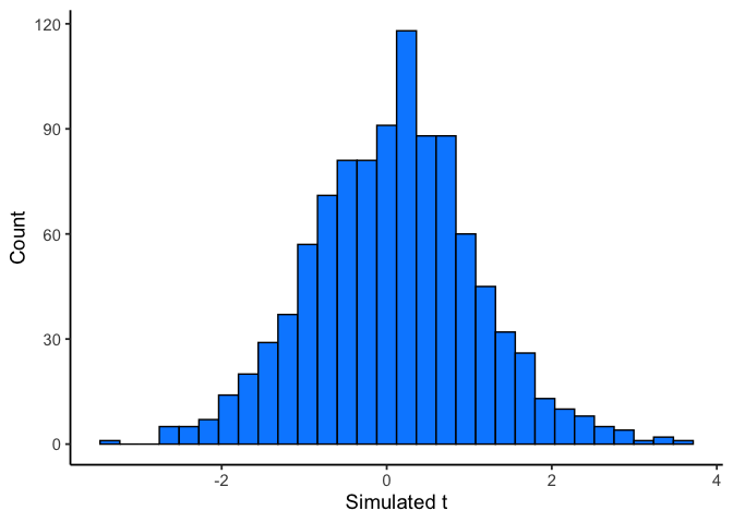
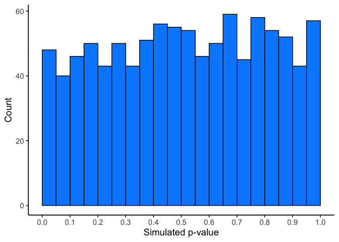
The simulated \(t\) distribution looks like a \(t\) distribution should, and it shows us how often we get \(t\) values of particular sizes. The \(p\)-distribution is flat under the null, which we are simulating here. This means you have the same chance of getting a \(t\) with a p-value between 0 and 0.05 as you would of getting one between .90 and .95. Those ranges are both ranges of 5%, so they hold an equal share of the \(t\) values by definition.

You can write the same simulation more compactly with replicate() instead of a for loop; it produces the same two distributions above:

simulated_ts <- replicate(1000, t.test(rnorm(30, 50, 25), mu = 50)$statistic)
simulated_ps <- replicate(1000, t.test(rnorm(30, 50, 25), mu = 50)$p.value)

6.6.2 The same machinery, other designs

The paired and independent-samples cases behave the same way, because they use the same \(t\) calculation on different inputs. A paired test runs a one-sample \(t\) on the difference scores; an independent-samples test swaps in the pooled standard error. Simulate either one under \(H_0\) and you get the same two pictures: a \(t\) distribution centered on zero, and a flat \(p\) distribution.

To adapt the code above, change only the line that generates the data:

# paired: one sample of difference scores
d <- rnorm(10, 0, 5) - rnorm(10, 0, 5)
t.test(d, mu = 0)$p.value

# independent samples: two separate groups
t.test(rnorm(10, 10, 5), rnorm(10, 10, 5), var.equal = TRUE)$p.value

What happens if there is a real difference in the simulated data? Let’s set one condition to have a larger mean than the other:

save_ps <- numeric(1000)
save_ts <- numeric(1000)
for ( i in 1:1000 ){
  condition_A <- rnorm(10,10,5)
  condition_B <- rnorm(10,13,5)
  differences <- condition_A - condition_B
  t_test <- t.test(differences, mu=0)
  save_ps[i] <- t_test$p.value
  save_ts[i] <- t_test$statistic
}

Figure 6.12: 1000 ps when there is a true difference

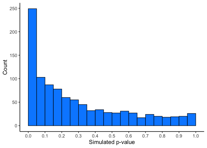
Now you can see that the \(p\)-value distribution is right-skewed: most of the values pile up near 0, with a long tail toward 1. This is because when there is a true effect, you will get p-values that are less than .05 more often. That happens because a true effect produces larger \(t\) values than you would get with no difference.

In this case, we wouldn’t be making a type I error if we rejected the null when p was smaller than .05. How many times would we do that out of our 1000 experiments?

length(save_ps[save_ps<.05])
#> [1] 249
length(save_ps[save_ps<.05])/1000
#> [1] 0.249

We got 249 simulations where p was less than .05, or 24.9% of experiments. A design that rarely detects a real effect needs to be improved before you run it.

The most direct lever is \(n\), the number of subjects. Let’s increase \(n\) from 10 to 100 and see what happens to the number of “significant” simulated experiments.

save_ps <- numeric(1000)
save_ts <- numeric(1000)
for ( i in 1:1000 ){
  condition_A <- rnorm(100,10,5)
  condition_B <- rnorm(100,13,5)
  differences <- condition_A - condition_B
  t_test <- t.test(differences, mu=0)
  save_ps[i] <- t_test$p.value
  save_ts[i] <- t_test$statistic
}

Figure 6.13: 1000 ps for n =100, when there is a true effect

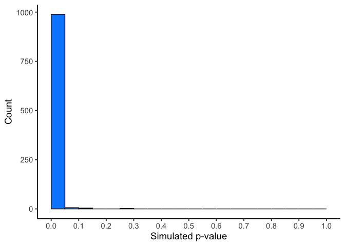
Now almost all of the experiments (988 of 1000) show a \(p\)-value of less than .05 (using a two-tailed test, the default in R). You can use this simulation process to determine how many subjects you need to reliably detect your effect.

6.7 Chapter Summary

Why it matters. The \(t\)-test is the first real inferential test in this course, and the logic it runs on, a signal measured against the noise around it, is the same logic behind ANOVA, regression, and everything else that follows.

Core ideas

• Signal over noise. A difference is only impressive relative to the variability around it. Every \(t\) statistic is a ratio: the effect you observed on top, an estimate of how much that effect could bounce around by chance on the bottom.
• Three forms, one idea. The one-sample, paired, and independent-samples \(t\)-tests differ in what goes into the numerator, but all three ask whether an observed difference is large compared to its own standard error. The paired test is just the one-sample test applied to difference scores.
• Why \(t\) and not \(z\). When the population SD \(\sigma\) is unknown, we estimate it with \(s\), which adds uncertainty. The \(t\) distribution accounts for that by being fatter in the tails than the normal, and it tightens toward the normal as degrees of freedom grow.
• Assumptions come in two kinds. Independence and a sound study design apply to every test in this book and are assumed from here on. The test-specific assumption for these tests is approximate normality, of the outcome for a one-sample test or of the difference scores for a paired test, or of each group, plus similar variances, for an independent-samples test.
• How worried to be depends on \(n\). Thanks to the Central Limit Theorem, \(t\)-tests are fairly robust to non-normality once samples are reasonably large. \(t\)-tests are least trustworthy when samples are small and skewed, which describes a lot of environmental field data. Plot your data first, and treat a Shapiro-Wilk result as evidence rather than a gate, since it has the least power with small samples, when a violation matters most.
• Choose your tails before you look. Default to two-tailed. Reserve one-tailed tests for cases where a difference in the opposite direction would lead to the same action as no difference, and decide before seeing the result.

Student, A. 1908. “The Probable Error of a Mean.” Biometrika 6: 1–2.

Welch, B. L. 1947. “The Generalization of ‘Student’s’ Problem When Several Different Population Variances Are Involved.” Biometrika 34: 28–35.