8  ANOVA

Some history first (Salsburg 2001). Sir Ronald Fisher invented the ANOVA and wanted to publish it in the journal Biometrika. The editor at the time was Karl Pearson, of Pearson’s \(r\), and the two men disliked each other, so Pearson refused to publish the new test. Fisher published it in the Journal of Agricultural Science instead. The feud carried into the next generation: years later, Karl Pearson’s son Egon Pearson, working with Jerzy Neyman, revamped Fisher’s ideas and re-cast them into what we now call null vs. alternative hypothesis testing. Fisher objected to that too.

8.1 ANOVA is Analysis of Variance

ANOVA stands for Analysis Of Variance. It tests whether differences among several group means are larger than we’d expect from chance alone.

With two groups, a \(t\)-test already answers that question. ANOVA extends the same logic to three or more groups, which comes up constantly in environmental science: multiple sites, multiple treatments, multiple time periods.

8.1.1 Why not just run multiple t-tests?

Suppose we’re comparing three restoration treatments for vegetation cover: compost, mulch, and a bare-soil control. With three groups, there are three possible pairwise comparisons: compost vs. mulch, compost vs. control, and mulch vs. control.

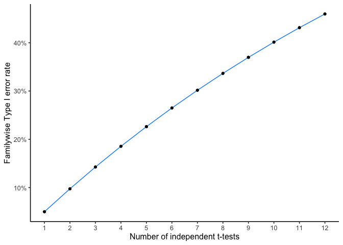
We could run a separate \(t\)-test for each. The problem is that every test carries its own 5% chance of a false positive, and those chances accumulate across tests. This follows from the independence multiplication rule in Chapter 3: if we run \(m\) independent tests at \(\alpha=.05\), the probability of at least one false positive across all of them is

\[P(\text{at least one false positive}) = 1-(1-\alpha)^m.\]

With three groups, that’s three tests and a familywise error rate of 14%, not 5%:

\[1-(1-.05)^3 = .14.\]

Number of groups (\(k\))	Pairwise tests (\(m\))	Familywise error rate
3	3	\(1-.95^3=.14\)
4	6	\(1-.95^6=.26\)
5	10	\(1-.95^{10}=.40\)

Even with only five groups, there’s a 40% chance of turning up at least one “significant” difference somewhere purely by chance, even if every population mean is identical. Figure 8.1 shows this inflation directly: as the number of independent \(t\)-tests grows, so does the chance that at least one is a false positive.

Figure 8.1: Familywise Type I error rate as the number of independent t-tests increases, at alpha = .05 per test.

ANOVA solves this by replacing many separate \(t\)-tests with one test that controls the overall error rate. It asks a single question:

\[H_0: \mu_1=\mu_2=\mu_3 \qquad H_a: \text{at least one mean differs}\]

Just like the \(t\)-test, different research designs call for different kinds of ANOVA: a one-way (between-subjects) ANOVA when every unit is measured once, and a repeated-measures ANOVA when the same units are measured under multiple conditions. This chapter covers the one-way case and ends with a short look at repeated measures; Chapter 10 extends the one-way case to two factors.

8.2 One-way ANOVA

The one-way ANOVA (also called a between-subjects or independent-factor ANOVA) is the simplest version of the test: one independent variable with two or more levels, and every unit measured once.

With exactly two groups, a \(t\)-test and a one-way ANOVA give the same answer: \(t^2=F\). Both compare the size of an effect to the amount of variation you’d expect from sampling error alone. The \(t\)-test expresses that comparison as \(t\), and the ANOVA expresses the same ratio as \(F\) (named for Fisher, its inventor).

\[F = \frac{\text{measure of effect}}{\text{measure of error}}\]

The difference is that \(F\) uses variances for both the numerator and the denominator, so \(F\) is a ratio of two variances: the variance you can explain (differences between group means) over the variance you can’t (leftover noise within each group).

\[F = \frac{\text{Can explain}}{\text{Can't explain}}\]

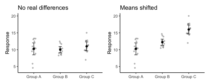
When the two are about the same size, \(F\approx 1\): group differences are no bigger than ordinary sampling noise. When explained variance is much larger than unexplained variance, \(F\) climbs well above 1, which is evidence that the groups differ. When it’s smaller, \(F\) drops below 1. An \(F\) of 5 means the group means are spread out five times more than the noise within groups would spread them on its own. An \(F\) of 0.6 means they are spread out less than that noise alone would typically produce.

Figure 8.2 shows both situations with the same noise. On the left, the group means differ by no more than the scatter within each group would produce. On the right, the means are separated by much more than that scatter. \(F\) measures that separation relative to the within-group scatter.

Figure 8.2: The same within-group noise with no real differences (left) and with the group means shifted (right). Three groups of 12; small points are individual scores, large dots are group means, bars are 95% confidence intervals.

8.2.1 Computing the \(F\)-value

ANOVA splits the total variation in the data into two sources: variation between groups, which group membership can explain, and variation within groups, which it can’t. If we can measure those two parts separately, we can turn them into a ratio and get an \(F\)-value.

\[\text{Total variation} = \text{Variation between groups} + \text{Variation within groups}\]

To make that precise we need an actual measure of variation. As in Chapter 2, that’s the sums of squares:

\[SS_\text{Total} = SS_\text{Between} + SS_\text{Within}\]

8.2.2 SS Total

\(SS_\text{Total}\) captures all of the variation in a dataset: the difference between each score and the grand mean, squared and summed. Writing \(Y_{ij}\) for score \(i\) in group \(j\) and \(\bar{Y}_\text{grand}\) for the grand mean,

\[SS_\text{Total} = \sum (Y_{ij} - \bar{Y}_\text{grand})^2.\]

Suppose we have three groups, A, B, and C, with 3 scores in each:

groups	scores	diff	diff_squared
A	20	13	169
A	11	4	16
A	2	-5	25
B	6	-1	1
B	2	-5	25
B	7	0	0
C	2	-5	25
C	11	4	16
C	2	-5	25
Sums	63	0	302
Means	7	0	33.56

The data are in long format, so each row is a single score. The mean of all of the scores is the Grand Mean, calculated in the table as 7.

The diff column holds every score’s distance from the grand mean; diff_squared squares those distances. Squaring matters because the raw differences sum to zero (the mean is the balancing point of the data), so working with them directly wouldn’t tell us anything. Squaring turns every deviation positive and, as a side effect, weights larger deviations more heavily.

Adding up all of the squared deviations gives the sum of squares (SS) from Chapter 2. Here \(SS_\text{Total} = 302\), the first piece of the partition:

\[SS_\text{Total} = SS_\text{Between} + SS_\text{Within}, \qquad 302 = SS_\text{Between} + SS_\text{Within}.\]

We only need to compute one of the two remaining pieces directly; the other follows by subtraction.

8.2.3 SS Between

\(SS_\text{Total}\) captured all of the variation in the data. \(SS_\text{Between}\) isolates the piece of that variation we can explain by group membership: how far each group’s mean sits from the grand mean.

To find it, replace every score with its own group’s mean, then square and sum each group mean’s distance from the grand mean. Writing \(\bar{Y}_j\) for the mean of group \(j\) and \(n_j\) for its number of scores,

\[SS_\text{Between} = \sum_j n_j(\bar{Y}_j - \bar{Y}_\text{grand})^2.\]

The \(n_j\) is there because every score in group \(j\) is replaced by the same group mean, so each group’s squared distance counts once per score. Here every group has 3 scores; with unequal groups, larger groups count more.

groups	scores	means	diff	diff_squared
A	20	11	4	16
A	11	11	4	16
A	2	11	4	16
B	6	5	-2	4
B	2	5	-2	4
B	7	5	-2	4
C	2	5	-2	4
C	11	5	-2	4
C	2	5	-2	4
Sums	63	63	0	72
Means	7	7	0	8

The new means column replaces each score with its group mean. Group A’s mean is 11, so there are three 11s, one per observation in group A. Groups B and C both average to 5, so the rest of the column is 5s.

Each score has been replaced by its own group’s mean, so within a group every value is now identical. Replacing scores this way throws away the individual variation inside each group and keeps only the differences between groups, which is what \(SS_\text{Between}\) measures.

Finding the differences between each of those group-mean values and the grand mean, squaring them, and summing gives \(SS_\text{Between} = 72\): the variation we can explain by group membership.

\(SS_\text{Between}\) can never be larger than \(SS_\text{Total}\), and indeed 72 is smaller than 302.

8.2.4 SS Within

We already have \(SS_\text{Total} = 302\) and \(SS_\text{Between} = 72\), so we can solve for \(SS_\text{Within}\) by subtraction:

\[SS_\text{Within} = SS_\text{Total} - SS_\text{Between} = 302 - 72 = 230.\]

We can also calculate \(SS_\text{Within}\) directly from the data, both to see where it comes from and to check the subtraction.

\[SS_\text{Within} = \sum (Y_{ij} - \bar{Y}_j)^2\]

groups	scores	means	diff	diff_squared
A	20	11	-9	81
A	11	11	0	0
A	2	11	9	81
B	6	5	-1	1
B	2	5	3	9
B	7	5	-2	4
C	2	5	3	9
C	11	5	-6	36
C	2	5	3	9
Sums	63	63	0	230
Means	7	7	0	25.56

This time, for each score we found the group mean first, then found the leftover error in that estimate: the diff column is the difference between each score and its own group mean, and diff_squared squares those differences. Summing them gives another sum of squares, \(SS_\text{Within}\): the deviations the group means can’t explain.

\(SS_\text{Within}\) has several other names. It is also called the error sum of squares, since it is the variation left over after group membership has explained what it can. R labels its row Residuals, and a results sentence reports \(MS_\text{Within}\) as \(MSE\) (mean squared error). All of these name the same quantity.

8.2.5 Degrees of freedom

Degrees of freedom work the same way here as for the \(t\)-test: every time we estimate something from the data, we use up a degree of freedom.

\(df_\text{Between} = k-1\), where \(k\) is the number of groups. With \(k=3\), \(df_\text{Between}=3-1=2\): once we fix the grand mean, two of the three group means are free to be anything, but the third is determined by the other two.

\(df_\text{Within} = N-k\), where \(N\) is the total number of scores. With \(N=9\) and \(k=3\), \(df_\text{Within}=9-3=6\): estimating each of the 3 group means uses up 3 degrees of freedom, so only 6 of the 9 individual deviations are free to vary.

\(df_\text{Total} = N-1\), and it splits the same way the sums of squares do: \(df_\text{Total} = df_\text{Between} + df_\text{Within}\), here \(8 = 2 + 6\).

8.2.6 Mean Squares

We’re building toward \(F=\dfrac{\text{measure of effect}}{\text{measure of error}}\), and it’s tempting to just divide \(SS_\text{Between}\) by \(SS_\text{Within}\) directly. The problem is that \(SS_\text{Within}\) sums over all 9 individual scores while \(SS_\text{Between}\) sums over only 3 group means, so \(SS_\text{Within}\) is almost always the much larger number, and the raw ratio wouldn’t be interpretable the way \(t\) or \(z\) are.

The fix is to convert each sum of squares into an average, or mean square, by dividing by its degrees of freedom (rather than its raw count, since these are estimated quantities):

\[MS_\text{Between} = \frac{SS_\text{Between}}{df_\text{Between}} = \frac{72}{2} = 36\]

\[MS_\text{Within} = \frac{SS_\text{Within}}{df_\text{Within}} = \frac{230}{6} = 38.33\]

Both are variances: \(MS_\text{Between}\) measures how much the group means vary, and \(MS_\text{Within}\) measures how much individual scores vary around their own group’s mean.

8.2.7 Calculate F

With \(MS_\text{Between}\) and \(MS_\text{Within}\) in hand, \(F\) is their ratio:

\[F = \frac{MS_\text{Between}}{MS_\text{Within}} = \frac{36}{38.33} = 0.94\]

8.2.8 The ANOVA table

All of these pieces, the \(df\)s, \(SS\)es, \(MS\)es, and finally \(F\), are conveniently organized into an ANOVA table:

Source	df	SS	MS	F	p
groups	2	72	36.00	0.94	0.442
Residuals	6	230	38.33

R labels the two rows groups (the between-groups row: what the means can explain) and Residuals (the within-groups row: what they can’t). Other software uses slightly different labels for the same two rows. The table adds no new information beyond what we already computed. It organizes the numbers, and \(MS_\text{Between}\) (36) divided by \(MS_\text{Within}\) (38.33) gives the \(F\)-value.

8.3 What does F mean?

Every number in the ANOVA table so far was computed directly from the data, except one: the \(p\)-value. Its meaning is the same as for any other test we’ve covered: the probability of observing an \(F\) this large or larger if the null hypothesis (no real group differences) were true.

Since \(F\) is a sample statistic, we can find out how it behaves the same way we found out how \(t\) behaves: simulate it many times under the null and look at the resulting distribution.

To build intuition for the F distribution, consider a simulated monitoring study with three site types (A, B, C). Each site type has 10 sampling plots, for 30 total. We measure species abundance at each plot. The null scenario applies: all 30 plots are drawn from the same null population distribution (mean = 100, \(\sigma\) = 10), so site type has no real effect on abundance. Any differences between group means arise from sampling error alone.

We run this simulation 10,000 times. Each time we compute F from the sample data. The histogram of those 10,000 F-values, shown in Figure 8.3, is the null distribution of F for this design.

Figure 8.3: A simulation of 10,000 experiments from a null population distribution with no group differences. The histogram shows 10,000 \(F\)-values, one for each simulation. These are values that F can take in this situation. All of these \(F\)-values were produced by random sampling error.

This \(F\) distribution has two properties. First, it never goes below 0: \(F\) is a ratio of two variances, and variances can’t be negative, so neither can \(F\). Second, it isn’t normal or symmetric; it’s right-skewed, and its exact shape depends on the numerator and denominator degrees of freedom.

Most simulated \(F\)-values here fall near or below 1, because under the null the two mean squares estimate the same thing. All 30 plots come from one null population distribution with \(\sigma = 10\). \(MS_\text{Within}\) estimates \(\sigma^2\) from the spread of scores inside each group. \(MS_\text{Between}\) estimates the same \(\sigma^2\) from how far the group means stray from the grand mean, since with no real effect, sampling variation is the only thing moving them. Two estimates of one variance give a ratio near 1. When the population means really differ, \(MS_\text{Between}\) picks up those differences on top of \(\sigma^2\), and \(F\) grows. Values reaching up toward 5 do occur, but the histogram shows they are rare. Every \(F\) here was produced purely by random sampling error, since we built the simulation with no real group differences at all.

8.3.1 Making decisions

We can use this null distribution of \(F\) to decide when a real experiment’s result is too large to be explained by chance:

1. Set \(\alpha = .05\).
2. Find the critical value of \(F\) for our design’s numerator and denominator \(df\)s.

Figure 8.4 marks that critical value on the histogram:

Figure 8.4: The critical value for \(F\) where 5% of all \(F\)-values lie beyond this point

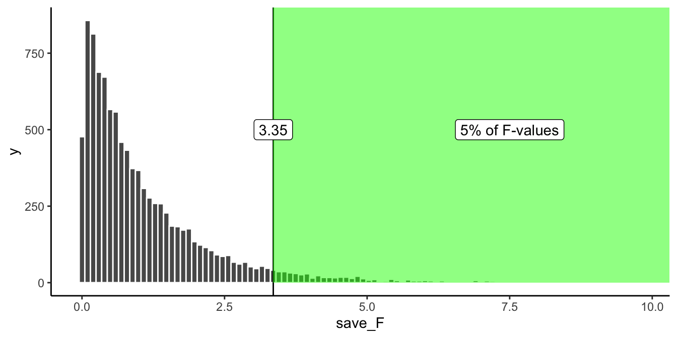
Only 5% of \(F\)-values from this null distribution are 3.35 or larger. That gives us a decision rule: if we ran the same design for real (30 plots, 10 per site type), we could treat \(F\geq3.35\) as evidence that the differences between site types are larger than chance would produce. An observed \(F\) of 3.4, for instance, would occur less than 5% of the time under the null, so seeing it would lead us to reject the null and conclude that site type mattered.

8.3.2 F and the means

An \(F\)-value and its \(p\)-value don’t, by themselves, tell us what the group means actually were. If a study reports \(F(2,27)=6.0\), \(p=.007\), we know only that an \(F\) this large would happen by chance less than 1% of the time. We still don’t know which means differed, or by how much, without looking at the group means directly (the ANOVA table itself doesn’t report them).

A large \(F\) with a small \(p\)-value does tell us one thing: we have evidence that the group means differ somewhere, because the variance explained by group membership (the numerator of \(F\)) is large relative to the variance within groups. Finding which means differ requires a separate step.

ANOVA is an omnibus test.

This is why ANOVA is called an omnibus test: omnibus meaning “comprising several items.” It answers one overall question that stands in for several pairwise ones at once.

With three groups A, B, and C, there are three possible pairwise differences: A vs. B, B vs. C, and A vs. C. We could test each with a separate \(t\)-test, or ask the more general omnibus question with a single ANOVA:

Hypothesis of no differences anywhere: \(A=B=C\)

Any differences anywhere:

1. \(A\neq B=C\) (A differs)
2. \(B\neq A=C\) (B differs)
3. \(C\neq A=B\) (C differs)
4. \(A\neq B\), \(B\neq C\), and \(A\neq C\) (all three differ)

A small \(F\) with a large \(p\)-value means we don’t reject the hypothesis of no differences: we have no evidence the three group means differ, and whatever gaps exist could easily be chance. A large \(F\) with a small \(p\)-value (below \(\alpha\)) means we reject that hypothesis and conclude at least one group mean differs from the others. That’s the omnibus test: it tells us whether the means differ, not yet which ones.

What group means look like when F exceeds the critical value.

The 10,000 simulated experiments never showed the group means behind each \(F\)-value. Earlier we found a critical value of 3.35: only 5% of \(F\)-values from this null distribution exceed it. Figure 8.5 shows the group means for 10 simulations with \(F>3.35\). Every one of them was still drawn from the same null population distribution, with no real group differences. Rejecting the null whenever \(F\) clears 3.35 is the right long-run decision rule, but every one of these particular simulations would be a Type I error if we did.

Figure 8.5: Different patterns of group means under the null when F is above critical value (these are all type I Errors).

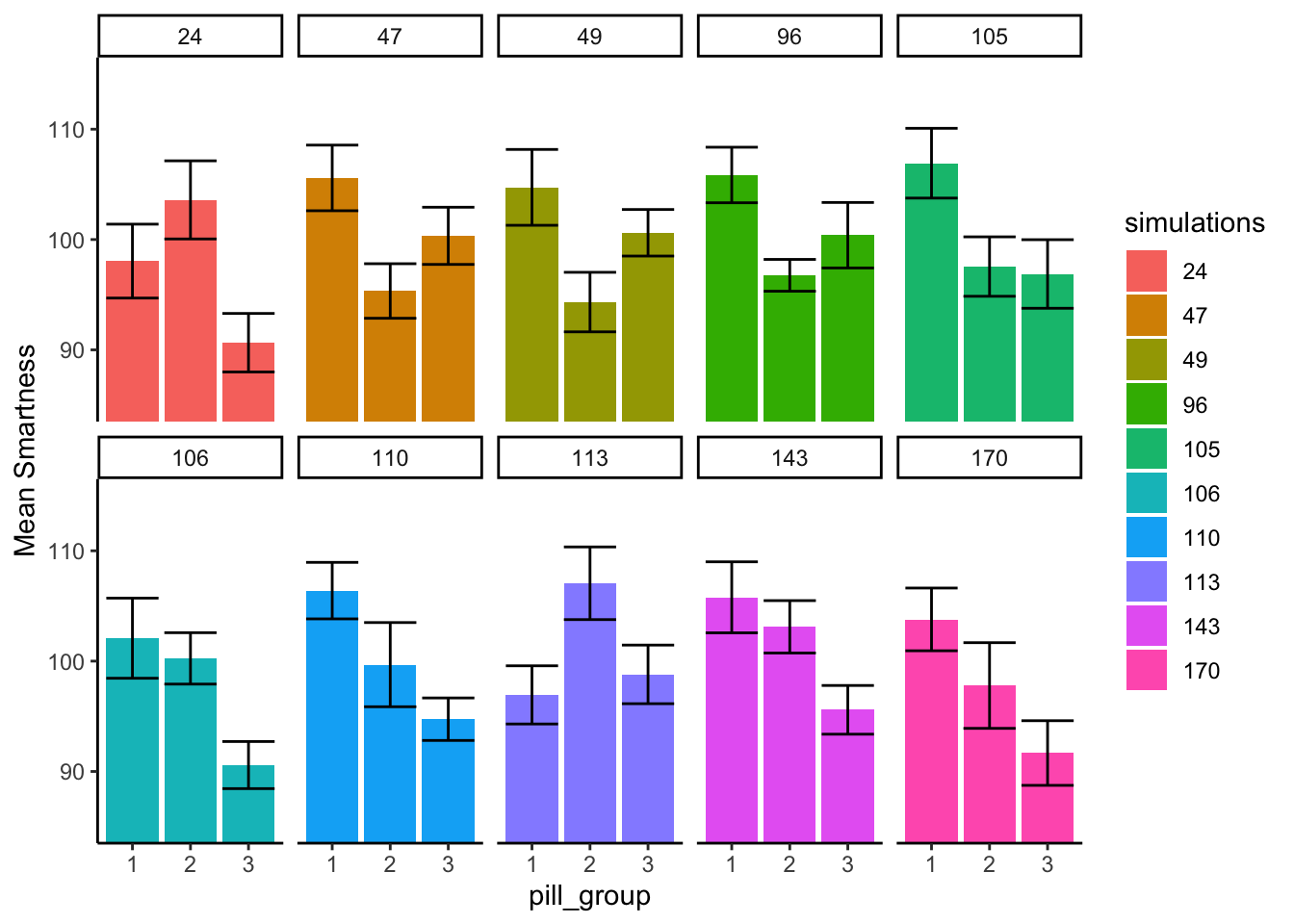
Every panel of Figure 8.5 now shows at least one group mean whose error bars don’t overlap with another’s: a visually convincing “real” difference. All ten are Type I errors. When this happens by chance, the data show a pattern, the \(F\)-value is large, and the \(p\)-value is small. A Type I error looks exactly like a real effect, and nothing in the output distinguishes them.

8.4 ANOVA on Real Data

We’ve covered the fundamentals of ANOVA: how to compute an \(F\)-statistic from the data, and how to interpret it along with its \(p\)-value. In practice, software handles these calculations for you, but you still need to know what the numbers mean to interpret them correctly. That is why we computed one ANOVA by hand.

The following example applies the full ANOVA workflow, from descriptive summaries through the omnibus F test to post-hoc comparisons, to a real ecological dataset. This is the same dataset used in Lab 11.

8.4.1 Salamander abundance across forest types

Plethodontid salamanders are sensitive indicators of forest condition: they depend on moist microhabitats, abundant coarse woody debris, and stable soil temperatures, all features that decline with forest disturbance. A field ecologist surveys salamander abundance across three forest types, laid out in Figure 8.6.

Figure 8.6: The salamander study as a design schematic. Structurally this is the two-group design from Chapters 4 and 6 with one more box added.

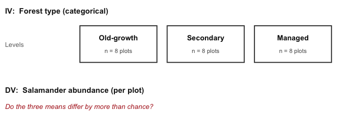
Compare that with the two-group designs earlier in the book: nothing has changed except the number of groups. That is why ANOVA is a generalization of the \(t\)-test. More groups also means more pairwise comparisons, which is the multiple-comparisons problem from the start of the chapter.

Let’s look at the data. You will work through these steps yourself in Lab 11.

Figure 8.7: Mean salamander abundance (individuals per plot) across three forest types. Points show individual plot counts; error bars show ±1 SE.

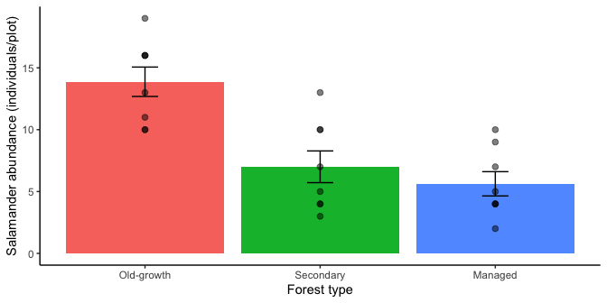
The bar graph shows a clear gradient: old-growth plots have the highest mean abundance, managed plantations the lowest, with secondary forest in between. The individual plot counts (dots) show considerable within-group variability, a reminder that even where a real difference exists, individual plots can vary substantially.

8.4.2 Checking ANOVA’s assumptions

Before running the ANOVA, check whether its assumptions hold. (Recall from Chapter 6 that independence is the universal assumption that applies to every test we cover and won’t be re-listed here; what follows are ANOVA’s test-specific assumptions.)

ANOVA has two: homogeneity of variance (the groups’ spread around their own means should be roughly comparable) and approximately normal residuals (each plot’s count minus its forest type’s mean, the same deviations that make up \(SS_\text{Within}\), should be roughly bell-shaped). Both matter because the \(F\)-test pools the within-group spread of every group into one error variance, \(MS_\text{Within}\), and then compares \(F\) to a null distribution that assumes normal residuals. Pooling only makes sense when the groups have similar spread.

Levene's test for homogeneity of variance

Statistic (F)	p-value	df	df residual
0.52	0.599	2	21

Shapiro-Wilk test on ANOVA residuals

Statistic (W)	p-value	Method
0.93	0.078	Shapiro-Wilk normality test

Levene’s test (Levene 1960; Brown and Forsythe 1974) gives \(F(2,21) = 0.52\), \(p = .60\): no evidence of unequal variance across forest types. The Shapiro-Wilk test (Shapiro and Wilk 1965) on the model’s residuals gives \(W = 0.93\), \(p = .078\): no evidence against normality either. Both checks are consistent with the individual plots in Figure 8.7: similar spread across groups, no glaring outliers.

A word of caution about formal assumption tests. It’s tempting to treat Levene’s test as a strict gate, where significant means “stop” and not significant means “proceed.” Resist that. With a small sample (exactly when a violated assumption matters most), these tests have low power and will often say “no problem” even when there is one. With a very large sample (where ANOVA is fairly robust to mild violations anyway), they have high power and will flag trivial differences as “significant.” A formal test is one piece of evidence, not the whole verdict, so look at the diagnostic plots too and use judgment. In practice, one-way ANOVA is moderately robust to mild departures from these assumptions, especially with balanced group sizes like we have here (8 plots per forest type). Worry most when small, unbalanced samples come with visibly skewed data or very different spreads. In that case, the nonparametric alternative below is the better choice.

With the assumptions reasonable, we run the one-way ANOVA to test whether these differences are larger than expected by chance alone.

Table 8.1: One-way ANOVA table for salamander abundance by forest type.

Source	df	SS	MS	F	p
forest_type	2	312.58	156.29	14.60	< .001
Residuals	21	224.75	10.70

ImportantResults reporting: one-way ANOVA

Report the direction in plain language, the test statistic with both degrees of freedom, the error term, \(p\), and the effect size.

There was a significant effect of forest type on salamander abundance, \(F(2, 21) = 14.60\), \(MSE = 10.70\), \(p < .001\), \(\eta^2 = 0.58\).

The F-value of 14.60 falls far into the tail of the null distribution of \(F\) for df(2, 21): values this large arise by chance less than 0.1% of the time. We reject the null hypothesis that all three group means are equal.

8.4.3 Effect size: eta-squared

The \(F\)-test answers whether the group means differ by more than chance would produce. It says nothing about how much of the variation in salamander abundance forest type explains. Chapter 5 made the same distinction, where \(p\) told us whether a difference was detectable and Cohen’s \(d\) told us how large it was.

ANOVA’s effect size is eta-squared (\(\eta^2\)), and we already computed both of its ingredients when we partitioned the sums of squares:

\[\eta^2 = \frac{SS_\text{Between}}{SS_\text{Total}} = \frac{SS_\text{Between}}{SS_\text{Between} + SS_\text{Within}}\]

\(SS_\text{Between}\) is the variation the group means explain and \(SS_\text{Total}\) is all the variation there is, so \(\eta^2\) is the proportion of the total variation explained by the grouping variable. It runs from 0 to 1.

Table 8.2: Eta-squared for the effect of forest type on salamander abundance.

SS Between	SS Within	SS Total	Eta-squared
312.58	224.75	537.33	0.582

Here \(\eta^2 = 0.58\): forest type explains about 58% of the variation in salamander abundance across these 24 plots. The remaining 42% is within-group variation, the plot-to-plot differences that forest type alone cannot explain.

\(\eta^2\) is the same quantity as \(R^2\) in regression (Chapter 9), computed the same way. Both divide the total variation into a part the model explains and a part it leaves over, and report the explained part as a proportion of the total.

Interpreting the number. Cohen’s conventional benchmarks are \(\eta^2 = 0.01\) (small), \(0.06\) (medium), and \(0.14\) (large), so 0.58 is a substantial effect. Treat those cutoffs as rough orientation rather than a grading scale: what counts as a large effect depends entirely on the system you are studying. An \(\eta^2\) of 0.10 would be unremarkable in a controlled greenhouse experiment and notable in a field survey where dozens of uncontrolled factors also drive the response.

Why report it at all. \(p\)-values depend on sample size and \(\eta^2\) does not. Survey enough plots and a difference of half a salamander per plot will clear \(p < .05\) while explaining almost none of the variation. Reporting both keeps a statistically detectable result from being mistaken for an ecologically meaningful one.

8.4.4 Post-hoc comparisons with Tukey HSD

The omnibus F test tells us that at least one group mean differs, but not which pairs. To identify which forest types differ, we use Tukey’s Honestly Significant Difference (HSD) test (Tukey 1949). Tukey HSD controls the familywise error rate across all pairwise comparisons, making it the appropriate choice after a significant ANOVA.

Table 8.3: Tukey HSD post-hoc comparisons for salamander abundance by forest type.

	diff	lwr	upr	p adj
Secondary-Old-growth	-6.875	-10.998	-2.752	0.0011
Managed-Old-growth	-8.250	-12.373	-4.127	0.0002
Managed-Secondary	-1.375	-5.498	2.748	0.6825

Reading the table, column by column. Each row is one pairwise comparison, and there are three of them because three groups make three pairs.

• diff is the difference in group means, computed as the first group in the row label minus the second: Secondary-Old-growth is secondary minus old-growth.
• lwr and upr are the lower and upper bounds of the 95% confidence interval for that difference.
• p adj is the \(p\)-value after adjusting for the fact that you are making three comparisons at once. Because of this adjustment, running the three comparisons here does not carry the 14% familywise error rate we computed at the start of the chapter.

Watch the sign. The row Secondary-Old-growth has a diff of \(-6.875\), and that negative sign does not mean secondary forest has more salamanders. It means secondary minus old-growth is negative, so old-growth is the higher of the two, by 6.88 individuals per plot. Always translate the sign back into a sentence naming which group is larger before you write anything down.

The confidence interval and the \(p\)-value say the same thing. A pair differs significantly at \(\alpha = .05\) exactly when its 95% interval excludes zero. Check both columns against each other as a habit: Secondary-Old-growth runs from \(-11.00\) to \(-2.75\), entirely below zero, and its \(p\) is .0011. Managed-Secondary runs from \(-5.50\) to \(2.75\), straddling zero, and its \(p\) is .68. The two columns can never disagree, so if they seem to, you have misread a row.

So the three comparisons give:

• Old-growth vs. Secondary: old-growth is higher by 6.88 individuals/plot, \(p = .001\). Significant.
• Old-growth vs. Managed: old-growth is higher by 8.25 individuals/plot, \(p < .001\). Significant.
• Secondary vs. Managed: they differ by 1.38 individuals/plot, \(p = .68\). Not significant.

“Not significant” does not mean “the same.” Secondary and managed plantation differ by 1.38 salamanders per plot in this sample. That difference is real in the data. The test says that with eight plots per group, we cannot distinguish it from sampling noise. A larger study might well separate them. Report it as “we did not detect a difference,” never as “there is no difference.”

Compact letter display. Once you have more than three groups, a list of pairwise sentences gets unwieldy fast, so results are usually summarized with letters placed above each group. The rule is simple: groups that share a letter were not significantly different; groups sharing no letter were. Figure 8.8 puts the salamander results in that form.

Figure 8.8: Mean salamander abundance with Tukey letters. Old-growth carries an ‘a’ and differs from both other types; secondary and managed share a ‘b’, so they were not distinguishable from each other.

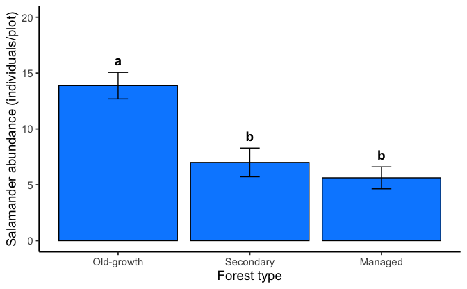
Old-growth gets its own letter because it differs from both of the others. Secondary and managed share a letter because the test could not separate them. Note that a group can carry two letters, written “ab”, when it differs from neither of two groups that do differ from each other. That looks contradictory but isn’t: it means that group sits in the middle, close enough to both ends that neither comparison reached significance, while the two ends are far enough apart that theirs did.

The pattern here is ecologically interpretable: old-growth forest supports the highest salamander abundance, consistent with its structural complexity and stable microclimate. Secondary forest and managed plantation could not be distinguished, suggesting that the early stages of forest recovery may not yet restore the conditions salamanders require.

8.4.5 Nonparametric alternative: the Kruskal-Wallis test

Our assumption checks above came back clean, so the ANOVA result stands as-is. But suppose they hadn’t: visibly unequal spread across groups, or clearly skewed residuals, especially with small or unbalanced samples. The Kruskal-Wallis test (Kruskal and Wallis 1952) is the nonparametric alternative to one-way ANOVA, in exactly the same relationship that the Mann-Whitney-Wilcoxon test has to the independent-samples \(t\)-test (in fact, Kruskal-Wallis is the Mann-Whitney-Wilcoxon logic extended to more than two groups).

How it works, conceptually. Rank every observation across all groups together, from smallest to largest, ignoring group membership. Then check whether the average rank differs more across groups than chance alone would produce. If forest type truly matters, one group’s observations should occupy systematically higher or lower ranks than the others.

Its assumption. Kruskal-Wallis does not require normality. Like the Mann-Whitney-Wilcoxon test, it is easiest to interpret as a test of differences in location (median) when the groups’ distributions have similar shape. If the shapes differ a lot, a significant result tells you the groups differ, but not whether that difference is in location, spread, or shape.

Kruskal-Wallis test on salamander abundance by forest type

Statistic (χ²)	p-value	df	Method
13.09	0.001	2	Kruskal-Wallis rank sum test

\(\chi^2(2) = 13.09\), \(p = .001\): significant, the same conclusion as the ANOVA (\(F(2,21)=14.60\), \(p<.001\)). The two tests agree, as expected when the parametric assumptions hold, as ours did here.

Post-hoc comparisons. Just as a significant ANOVA needs Tukey HSD to identify which groups differ, a significant Kruskal-Wallis result needs its own follow-up: pairwise rank-sum tests (Mann-Whitney-Wilcoxon, applied to each pair) with a correction for running multiple comparisons (Holm 1979).

Pairwise Mann-Whitney-Wilcoxon comparisons (Holm-adjusted)

Group 1	Group 2	p-value
Secondary	Old-growth	0.011
Managed	Old-growth	0.004
Managed	Secondary	0.486

The pattern matches Tukey HSD exactly: Old-growth differs significantly from both Secondary (\(p=.011\)) and Managed (\(p=.004\)), while Secondary and Managed do not differ from each other (\(p=.49\)). The two approaches use different assumptions and different calculations, and they agree here because the parametric assumptions held.

8.5 Repeated-measures ANOVA

Every unit in the salamander study was measured once: 24 plots, 8 per forest type. Many environmental studies instead measure the same units under every condition, such as the same monitoring stations in every season or the same streams before, during, and after a drought. That is a repeated-measures (within-subjects) design, and it calls for a repeated-measures ANOVA.

This is ANOVA’s version of the paired \(t\)-test from Chapter 6. The paired \(t\)-test subtracted each plot’s before score from its own after score, so differences between plots dropped out and only the change was left. With three or more conditions there is no single difference to take, so repeated-measures ANOVA does the equivalent with sums of squares: it measures how much the units differ from one another and removes that variation from the error term.

8.5.1 Fine particulate matter at four monitoring stations

An air quality agency has four PM2.5 monitors, ordered from the most rural (A) to the most urban (D). Table 8.4 gives each monitor’s mean PM2.5 concentration in winter, spring, and summer. The question is whether concentrations differ by season: \(H_0: \mu_\text{Winter}=\mu_\text{Spring}=\mu_\text{Summer}\) vs. \(H_a\): at least one seasonal mean differs.

Table 8.4: Seasonal mean PM2.5 (µg/m³) at four monitoring stations, with each station’s mean and each season’s mean.

Station	Winter	Spring	Summer	Station mean
A	9	2	4	5
B	9	8	7	8
C	16	11	12	13
D	18	11	13	14
Season mean	13	8	9	10

Winter is the highest season at every station. But the stations themselves differ far more than the seasons do. Station A averages 5 µg/m³ and station D averages 14.

8.5.2 Splitting off the stations

A one-way ANOVA on these 12 numbers would split the variation into two pieces, as before: \(SS_\text{Total} = 230\), \(SS_\text{Between} = 56\) for seasons, and \(SS_\text{Within} = 174\) left over. It would also break the independence assumption, because each station contributes three of the 12 numbers.

Repeated-measures ANOVA splits \(SS_\text{Within}\) one more time. Part of it is station-to-station variation, \(SS_\text{Subjects}\), computed exactly like \(SS_\text{Between}\) but from the station means instead of the season means. Each station mean counts once per season, so

\[SS_\text{Subjects} = 3\left[(5-10)^2 + (8-10)^2 + (13-10)^2 + (14-10)^2\right] = 3(54) = 162.\]

Whatever is left is the error term:

\[SS_\text{Error} = SS_\text{Within} - SS_\text{Subjects} = 174 - 162 = 12,\]

so the full split is

\[SS_\text{Total} = SS_\text{Between} + SS_\text{Subjects} + SS_\text{Error}, \qquad 230 = 56 + 162 + 12.\]

\(SS_\text{Error}\) is the part of the within-season variation that the stations’ own levels can’t explain: how much each station’s seasonal pattern departs from the average seasonal pattern. Its degrees of freedom are \((k-1)(n-1) = (3-1)(4-1) = 6\), where \(n\) is the number of stations. The stations use up 3 of the 9 degrees of freedom the one-way ANOVA would have had.

\(F\) uses the same numerator as before, \(MS_\text{Between} = 56/2 = 28\). Only the denominator changes:

\[\text{One-way: } F = \frac{28}{174/9} = \frac{28}{19.33} = 1.45 \qquad \text{Repeated measures: } F = \frac{28}{12/6} = \frac{28}{2} = 14.00\]

Removing the stations shrank the error mean square from 19.33 to 2, and \(F\) grew by the same factor. That is why a repeated-measures design has more power than a between-subjects design with the same number of measurements whenever the units differ from one another, as monitoring stations usually do: the unit-to-unit differences are no longer counted as noise. The repeated-measures test finds a significant seasonal effect, \(F(2, 6) = 14.00\), \(p = .005\). The one-way ANOVA would give \(F(2, 9) = 1.45\), \(p = .28\), and miss it.

8.6 Chapter Summary

Why it matters. Comparing more than two groups with a stack of \(t\)-tests inflates your false-positive rate fast. ANOVA solves that by asking one omnibus question first, and its variance-partitioning logic is the same idea that reappears in regression, factorial designs, and ANCOVA.

Core ideas

• Why not just run more \(t\)-tests. Each comparison carries its own chance of a false positive, and they accumulate: with \(m\) comparisons the familywise error rate is \(1-(1-\alpha)^m\), which is already 14% for three groups.
• Partition the variation. Total variation splits into a piece explained by group membership (\(SS_\text{Between}\)) and unexplained residual variation (\(SS_\text{Within}\)).
• \(F\) is a ratio of the two. After adjusting each sum of squares for its degrees of freedom, \(F = MS_\text{Between} / MS_\text{Within}\). A large \(F\) means between-group differences are large relative to within-group noise.
• Two steps, always in order. First the omnibus test: do any group means differ? Only if that is significant do you run post-hoc comparisons (Tukey HSD) to find out which pairs differ.
• \(\eta^2\) is the effect size. \(SS_\text{Between}/SS_\text{Total}\) is the proportion of variation explained by the grouping variable. It is the same quantity as regression’s \(R^2\), and it does not depend on sample size the way \(p\) does, so report it alongside \(F\).
• Check the assumptions. ANOVA needs approximately equal variances across groups (Levene’s test) and roughly normal residuals. Treat formal tests as evidence rather than a gate, since they have least power exactly when small samples make violations matter most.
• When assumptions fail. The Kruskal-Wallis test is the rank-based alternative, with pairwise.wilcox.test() as its post-hoc counterpart.
• Repeated measures. When the same units are measured under every condition, repeated-measures ANOVA splits \(SS_\text{Within}\) into \(SS_\text{Subjects}\) and a smaller \(SS_\text{Error}\). The smaller error term is why it has more power, the same reason the paired \(t\)-test does.

Brown, M. B., and A. B. Forsythe. 1974. “Robust Tests for Equality of Variances.” Journal of the American Statistical Association 69: 364–67.

Holm, S. 1979. “A Simple Sequentially Rejective Multiple Test Procedure.” Scandinavian Journal of Statistics 6: 65–70.

Kruskal, W. H., and W. A. Wallis. 1952. “Use of Ranks in One-Criterion Variance Analysis.” Journal of the American Statistical Association 47: 583–621. https://doi.org/10.1080/01621459.1952.10483441.

Levene, H. 1960. “Robust Tests for Equality of Variances.” In Contributions to Probability and Statistics: Essays in Honor of Harold Hotelling, edited by I. Olkin et al. Stanford University Press.

Salsburg, David. 2001. The Lady Tasting Tea: How Statistics Revolutionized Science in the Twentieth Century. Macmillan.

Shapiro, S. S., and M. B. Wilk. 1965. “An Analysis of Variance Test for Normality (Complete Samples).” Biometrika 52: 591–611.

Tukey, John W. 1949. “Comparing Individual Means in the Analysis of Variance.” Biometrics 5 (2): 99–114.